Stata Guide

Setup Requirements

Use CPL’s Stata Schemes and the correct font

Start your .do file with the following:

set scheme CPL_theme
graph set window fontface "Gill Sans Nova Book"

CPL’s Stata schemes save you time by setting the default color palette and display options for figures. These can be manually adjusted if needed.

There are three schemes: - CPL_theme uses the color palette of CPL’s policy briefs. This is your default scheme. - CPL_theme_Berkeley and CPL_theme_UCLA use university color palettes but are otherwise identical to CPL_theme

Scheme Installation

• Schemes are saved in the Commons at: \\COMMONS\commons\code\stata\00_cpl_theme\
• Copy these files to C:\users\YOURUSERNAME\ado\plus\c and Stata will recognize them when called

Saving Your Work

Use graph export to save your graphs.

graph export "FILENAME.EXTENSION", replace

Graphs can be exported as:

• .pdf: Portable Document Format
• .png: Portable Network Graphics
• .jpg: JPEG
• .eps: Encapsulated PostScript (good for embedding in LaTeX docs)

Additional image types supported, see help graph export for the full list.

Examples

This section provides nine customizable code templates for creating data visualizations with the twoway and graph bar functions in Stata.

All examples saved as separate templates in \\COMMONS\commons\code\stata\01_figure_guide\templates

Time Series with Legend

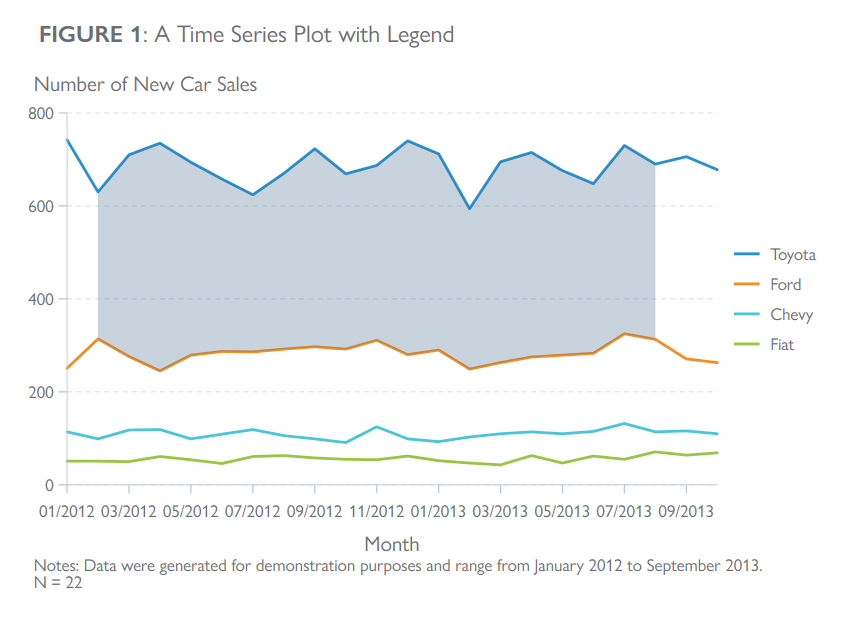
Here’s how to set up your data to label lines directly instead of using a legend.

1. Sort your data by the variable that will be used as the x-axis.

2. For each y-variable, create a new string variable. Leave every row of the new variable blank except for the last row. You will label the last row so that only the final “point” on your line graph will be labeled.

clear all
set more off

set scheme CPL_theme
graph set window fontface "Gill Sans Nova Book"

* Set root directory
global rootdir "\\COMMONS\commons\code\stata\01_figure_guide"

* Import raw data
use "$rootdir\data\figure_guide_data.dta", clear

*sort on x-variable
sort yearmonth

* Create local for y variable
local yvar "Toyota Ford Chevy Fiat"

* Use the variable name as the label, and add to the last observation of each y-variable. 
foreach var in `yvar'{
gen label_`var' = "`var'" if _n==_N
}

Your data will now look like this:

1. Now graph the data using twoway connected instead of twoway line, setting msize(0) to remove the markers you’d normally see in a scatter plot, and using mlab() to label your y-variables.

You may need to increase the right hand margin of your graph region to accommodate your labels by using graphregion(margin(r+#), or reposition your labels using the mlabposition() option with clock face positioning; eg 12 for above centered, 6 for centered below.

clear all
set more off

set scheme CPL_theme
graph set window fontface "Gill Sans Nova Book"

* Set root directory
global rootdir "\\COMMONS\commons\code\stata\01_figure_guide"

* Import raw data
use "$rootdir\data\figure_guide_data.dta", clear

* sort on x-variable
sort yearmonth

* Create local for y variable
local yvar "Toyota Ford Chevy Fiat"

* Add a label to the last observation of each y-variable. 
foreach var in `yvar'{
gen label_`var' = "`var'" if _n==_N
}

*Begin graphing

#delimit ;
twoway connected Toyota Ford Chevy Fiat yearmonth, 
        
        /*specify variable containing label for each Y variable in order*/
        mlab(label_Toyota label_Ford label_Chevy label_Fiat) 
        
        /*set the size of the marker for each Y variable to zero*/ 
        msize(0 0 0 0)                                                              
    
        /*increase right margin to accommodate labeling*/
        graphregion(margin(r+7))    

    /*add shading between lines for Toyota and Ford*/
    || rarea Toyota Ford yearmonth in 2/20,                                         
        color(navy%30) lwidth(0)                                                    

    /*set y-axis value labels*/
    ylabel(0(200)800, labsize(small))   

    /*use subtitle in 11 o'clock position for y axis title instead of repositioning ytitle*/
    subtitle("Number of New Car Sales", position(11) margin(b+2 l-6) size(medsmall))                        
        
    /*set x-axis value labels*/
    xlabel(624(2)645, format(%tm_NN/ccYY) labsize(small))   

    /*set x-axis title*/                                    
    xtitle("Month", margin(t+3 b-2)) 
    
    /*set graph title if in draft form, else add in destination document*/
    title("{bf: FIGURE 2}: A Time Series Plot with Line Labels",                            
        span position(11) size(medium)  margin(b+3 l+1))                        
                
    /*add figure note if in draft form, else add in destination document*/
    note("Notes: Data were generated for demonstration purposes and range from January 2012 to September 2013."                         
        "N = `c(N)'",                                               
        size(small)                                                         
        margin(t+2 l-6))            
    ;                                                                   
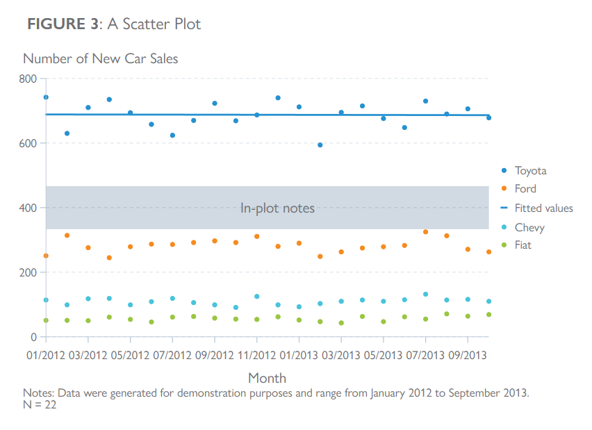
#delimit cr

Scatter Plots

clear all
set more off

set scheme CPL_theme
graph set window fontface "Gill Sans Nova Book"

* Set root directory
global rootdir "\\COMMONS\commons\code\stata\01_figure_guide"

* Import raw data
use "$rootdir\data\figure_guide_data.dta", clear

#delimit ;
/* initiate scatter plot with multiple Y variables listed before single X variable */
twoway scatter Toyota Ford Chevy Fiat yearmonth
    
    /*add linear fit line */
    || lfit Toyota yearmonth, lcolor("38 145 208") 
    
    /* create banded area at y=400 */
    yline(400, lpattern(solid) lwidth(10) lcolor(navy%20))                                          

    /* write note about importance of shaded region */
    text(400 635 "In-plot notes", color("109 110 113") size(medsmall))  

    /*set y-axis value labels*/
    ylabel(0(200)800, labsize(small))   

    /*use subtitle in 11 o'clock position for y axis title instead of repositioning ytitle*/
    subtitle("Number of New Care Sales", position(11) margin(b+2 l-6) size(medsmall))                       
        
    /*set x-axis value labels*/
    xlabel(624(2)645, format(%tm_NN/ccYY) labsize(small))   

    /*set x-axis title*/                                    
    xtitle("Month", margin(t+3 b-2))                                                        
        
    /* set up legend, arrange linear fit (5) key next to observational data key (2) */  
    legend(on position(3) cols(1) order(1 2 5 "Fitted values" 3 4) region(lwidth(0))                                
        symxsize(2) size(small))        

    /*set graph title if in draft form, else add title in destination document*/
    title("{bf: FIGURE 3}: A Scatter Plot",                         
        span position(11) size(medium)  margin(b+3 l+1))                        
                
    /*add figure note if in draft form, else add in destination document*/
    note("Notes: Data were generated for demonstration purposes and range from January 2012 to September 2013."                         
        "N = `c(N)'",                                               
        size(small)                                                             
        margin(t+1 l-6))                                                            
    ;                                                                   
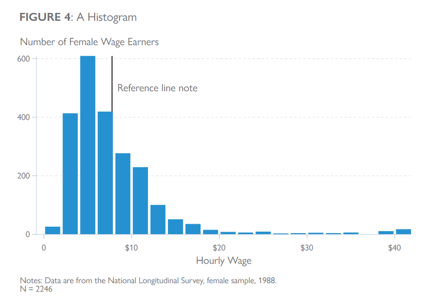
#delimit cr         

Histograms

clear all
set more off

set scheme CPL_theme
graph set window fontface "Gill Sans Nova Book"

* Import raw data.
sysuse nlsw88, clear

* twoway histogram doesn't automatically set bar colors according to scheme
* must be set manually.

#delimit ;

twoway hist wage,
    
    color("38 145 208") /*set bar color to CPL Policy Brief Blue*/
    width(2)            /*set width of bins*/
    start(0)            /*force bins to start at 0*/
    gap(15)             /*set gap between bars*/    
    frequency           /*request bins be frequency counts*/
    
    /*set y-axis value label size*/
    ylabel(,labsize(small))

    /*remove y-axis title*/
    ytitle("")
    
    /*use subtitle in 11 o'clock position for y axis title instead of repositioning ytitle*/
    subtitle("Number of Female Wage Earners", position(11) margin(b+2 l-6) size(medsmall))

    /*Specify x-axis title and position*/
    xtitle("Hourly Wage", margin(t+2))
    
    /*set x-axis labels with $ sign and set size*/
    xlabel(0 10 "$10" 20 "$20" 30 "$30" 40 "$40", labsize(small))   
    
    /*add reference line for mean*/
    xline(7.77, lpattern(solid) lcolor(black) )
    
    /*add note for reference line in y x location with compass direction orientation*/
    text(500 8 "Reference line note", placement(east)
    color("109 110 113") size(medsmall))
    

    /*set graph title if in draft form, else add title in destination document*/
    title("{bf: FIGURE 4}: A Histogram",                            
        span position(11) size(medium)  margin(b+3 l+1))                        
                
    /*add figure note if in draft form, else add in destination document*/
    note("Notes: Data are from the National Longitudinal Survey, female sample, 1988."                          
        "N = `c(N)'",                                               
        size(small)                                                         
        margin(t+2 l-6))
    ;
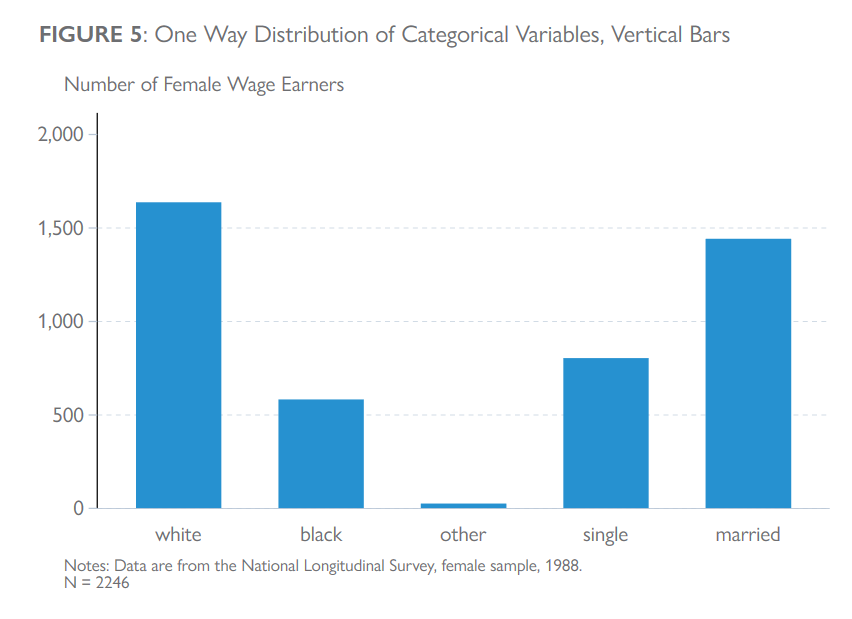
#delimit cr

Bar Graphs

Categorical Variables

clear all
set more off

set scheme CPL_theme
graph set window fontface "Gill Sans Nova Book"

* Import raw data.
sysuse nlsw88, clear

/*create dummy indicator variables from race and marital status variables*/
gen white = race == 1

gen black = race == 2

gen other = race == 3

rename married maritalstatus

gen single = maritalstatus == 0

gen married = maritalstatus == 1

#delimit ;

/*initialize command, set reporting statistic to sum of dummy variable within sample*/
graph bar (sum) 

    /*list all variables to be summed*/
    white black other single married, 
    
    /*treat variables as categories (see appendix tutorial)*/
    ascategory  

    /*use variable names instead of variable labels*/
    nolabel

    /*use subtitle in 11 o'clock position for y axis title instead of repositioning ytitle*/
    subtitle("Number of Female Wage Earners", position(11) margin(b+2 l-6) size(medsmall))  

    /*set graph title if in draft form, else add title in destination document*/
    title("{bf: FIGURE 5}: One Way Distribution of Categorical Variables, Vertical Bars",                           
        span position(11) size(medium)  margin(b+3 l+1))                        
                
    /*add figure note if in draft form, else add in destination document*/
    note("Notes: Data are from the National Longitudinal Survey, female sample, 1988."                          
        "N = `c(N)'",                                               
        size(small)                                                         
        margin(t+2 l-6))        
    ;
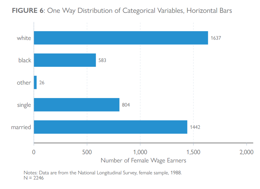
#delimit cr

Categorical, Horiztonal

clear all
set more off

set scheme CPL_theme
graph set window fontface "Gill Sans Nova Book"

* Import raw data.
sysuse nlsw88, clear

/*create dummy indicator variables from race and marital status variables*/
gen white = race == 1

gen black = race == 2

gen other = race == 3

rename married maritalstatus

gen single = maritalstatus == 0

gen married = maritalstatus == 1

#delimit ;

/*initialize command, set reporting statistic to sum of dummy variable within sample*/
graph hbar (sum) 

    /*list all variables to be summed*/
    white black other single married, 
    
    /*treat variables as categories (see appendix tutorial)*/
    ascategory  

    /*use variable names instead of variable labels*/
    nolabel

    /*add data value labels to ends of bars*/
    blabel(bar) 

    /*add axis title*/
    ytitle("Number of Female Wage Earners", size(medsmall) margin(t+2)) 

    /*set graph title if in draft form, else add title in destination document*/
    title("{bf: FIGURE 6}: One Way Distribution of Categorical Variables, Horizontal Bars",                         
        span position(11) size(medium)  margin(b+3 l+1))                        
                
    /*add figure note if in draft form, else add in destination document*/
    note("Notes: Data are from the National Longitudinal Survey, female sample, 1988."                          
        "N = `c(N)'",                                               
        size(small)                                                         
        margin(t+2 l-6))    
    ;
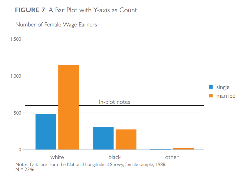
#delimit cr

Two-way Dist, Y-Axis count with Reference

clear all
set more off

set scheme CPL_theme
graph set window fontface "Gill Sans Nova Book"

sysuse nlsw88, clear

#delimit ;

/*initialize command, specify y variable if using, and display statistic*/
/*statistic can be count, percent, mean, median, sum pX, min, or max*/
/*when no statistic is specified, the default is mean */
graph bar (count), 
    /*first x variable*/
    over(married) 
    
    /*second x variable*/
    over(race) 
    
    /*treat x variables like y variables*/
    /*eg each level assigned different colors, group together on x axis*/
    /*and identify levels with a legend */
    asyvars 
    
    /*add a small gap between levels of first x variable*/
    bargap(10) 
    
    /*set y-axis to match theme*/   
    yscale(lcolor("184 198 214"))   

    /*set y-axis value label size*/
    ylabel(,labsize(small))                                                         
            
    /*use subtitle in 11 o'clock position for y axis title instead of repositioning ytitle*/
    subtitle("Number of Female Wage Earners", position(11) margin(b+2 l-6) size(medsmall))                      
    ytitle("")
    
    /*add reference line at y=600*/
    yline(600, lpattern(solid) lcolor(black))                                                           
    
    /*add text to describe reference line*/
    text(650 50 "In-plot notes", color("109 110 113") size(medsmall))   
    
    /*set legend options*/
    legend(on position(3) cols(1) region(lstyle(none))
        symysize(2)                                                         
        symxsize(2)) 

    /*set graph title if in draft form, else add title in destination document*/
    title("{bf: FIGURE 7}: A Bar Plot with Y-axis as Count",                            
        span position(11) size(medium)  margin(b+3 l+3))                        
                
    /*add figure note if in draft form, else add in destination document*/
    note("Notes: Data are from the National Longitudinal Survey, female sample, 1988."                          
        "N = `c(N)'",                                               
        size(small)                                                         
        margin(t+1 l-6))        
    ;
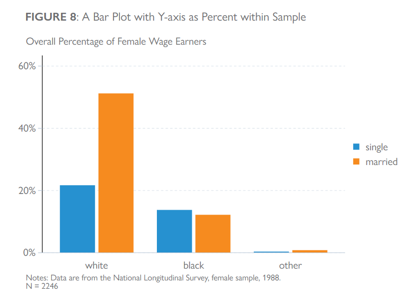
#delimit cr

Y-axis as Percent within Sample

clear all
set more off

set scheme CPL_theme
graph set window fontface "Gill Sans Nova Book"

* Import raw data.
sysuse nlsw88, clear

#delimit ;

/*initialize command, allow default reporting statistic; percent of group within sample*/
graph bar, 
    
    /*set specify variables to graph as counts*/
    over(married) over(race) 
    
    /*treat the "over" variables like "y variables" (see appendix tutorial)*/
    asyvars 
    
    /*add space between bars*/
    bargap(10) 
    
    /*set y-axis range*/
    yscale(range(0(20)60))
    
    /*label y-axis values with % sign*/
    ylabel(0 "0%" 20 "20%" 40 "40%" 60 "60%")
    
    /*use subtitle in 11 o'clock position for y axis title instead of repositioning ytitle*/
    subtitle("Overall Percentage of Female Wage Earners", position(11) margin(b+2 l-6) size(medsmall))                      
    ytitle("")
    
    /*add legend, suppress outline*/
    legend(on position(3) cols(1) region(lstyle(none)) 
        symysize(2)                                                         
        symxsize(2))

    /*set graph title if in draft form, else add title in destination document*/
    title("{bf: FIGURE 8}: A Bar Plot with Y-axis as Percent within Sample",                            
        span position(11) size(medium)  margin(b+3 l+3))                        
                
    /*add figure note if in draft form, else add in destination document*/
    note("Notes: Data are from the National Longitudinal Survey, female sample, 1988."                          
        "N = `c(N)'",                                               
        size(small)                                                         
        margin(t+1 l-6))    
    ;
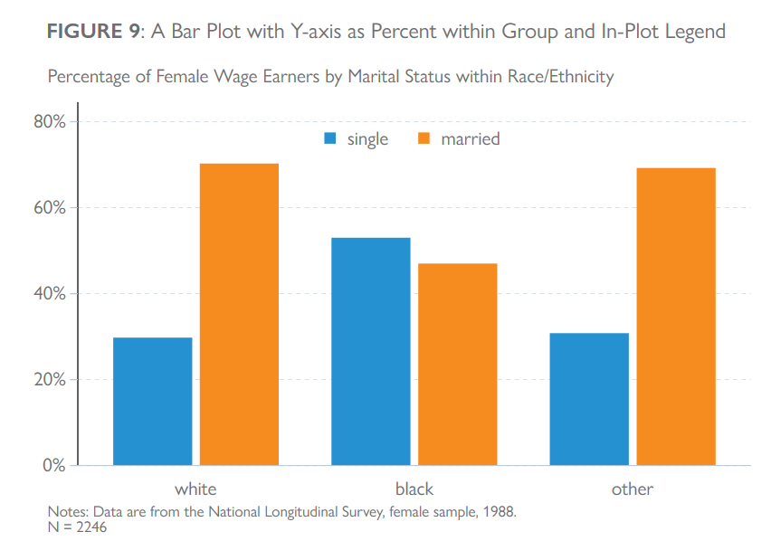
#delimit cr

Y-axis as Percent within Group and In Plot Legend

clear all
set more off

set scheme CPL_theme
graph set window fontface "Gill Sans Nova Book"

* Import raw data.
sysuse nlsw88, clear

#delimit ;

/*initialize command, allow default reporting statistic; percent of group within sample*/
graph bar, 
    
    /*specify variables to graph as counts*/
    over(married) over(race) 
    
    /*treat the "over" variables like "y variables" (see appendix tutorial)*/
    asyvars 
    
    /*report the percentage of the first "over" group within the second*/
    percentages 
    
    /*add space between bars*/
    bargap(10) 
    
    /*set y-axis range*/
    yscale(range(0(20)80))
    
    /*label y-axis values with % sign*/
    ylabel(0 "0%" 20 "20%" 40 "40%" 60 "60%" 80 "80%")
    
    /*use subtitle in 11 o'clock position for y axis title instead of repositioning ytitle*/
    subtitle("Percentage of Female Wage Earners by Marital Status within Race/Ethnicity", position(11) margin(b+2 l-6) size(medsmall))      
    ytitle("")
    
    /*add legend inside graph region, suppress outline, set legend fill to transparent*/
    legend(on position(12) ring(0) bmargin(t+2) rows(1) region(lstyle(none) fcolor(none)) 
        symysize(2) symxsize(2) )

    /*set graph title if in draft form, else add title in destination document*/
    title("{bf: FIGURE 9}: A Bar Plot with Y-axis as Percent within Group and In-Plot Legend",                          
        span position(11) size(medium)  margin(b+3 l+3))                    
                
    /*add figure note if in draft form, else add in destination document*/
    note("Notes: Data are from the National Longitudinal Survey, female sample, 1988."                          
        "N = `c(N)'",                                               
        size(small)                                                         
        margin(t+1 l-6))    
    ;
#delimit cr

Formatting Options for All Graphs

This section details universal options for formatting axes, text elements, legends, graph and plot regions for all graphs.

Axes formatting options

yscale and xscale: Control the Y and X axes scale and appearance

yscale(range() reverse alt log lcolor() off)

xscale(range() reverse alt log lcolor() off)

• off: Force axis suppression.

• range(): Specify axis range.

• log: Use logarithmic scale.

• alt: Place axis on side opposite to default in relation to plot (default is left for y axis and bottom for x axis).

• reverse: Control whether scale runs from min to max (default) or max to min.

• lcolor(): Set axis color. See help colorstyle. Default: 209 219 229 (RGB).

ylabel and xlabel: Control attributes of Y and X axes labels.

ylabel(min(gap)max, angle() format() labsize() nogrid)

xlabel(min(gap)max, angle() format() labsize() grid)

• min(gap)max,: Range and gap of labels; for example 0(10)100 will label the specified axis 0,10,20,30…100. Be consistent with scale values. Comma required if additional options specified.

• angle(): Set label angle (how much tilting). Default: 0 (horizontal).

• format(): Change formatting of values as shown on the axis. See help format and help datetime for numeric and date formatting codes.

• labsize(small): Set label size. See help textsizestyle for all sizes. Default: small.

• [no]grid: Remove horizontal gridlines to yscale (nogrid) or add vertical gridlines to xscale(grid). Default: grid for yscale, nogrid for xscale.

ytitle and xtitle: Create and format axis titles.

ytitle("Title", color() size() margin())

xtitle("Title", color() size() margin())

• “Title”,: Axis title. Blank by defult ("",). Comma required if additional options specified.

• color(): Set title color. See help colorstyle. Default: 109 110 113 (RGB).

• size(): Set font size. See help textsizestyle for all sizes. Default: small for ytitle, medsmall for xtitle.

• margin(): Set margin width around title. Suboptions include t(top), b(bottom), l(left), and r(right). Adjust by specifying =/+/-#, where # is % of minimum of width and height of the graph. Setting this usually takes some trial and error.

Text

title and subtitle: Graph title. Always use titles and figure numbers when drafting figures or during preliminary analyses. During publication titles will be added in the destination document.

Use left justified subtitles to create horizontal y-axis labels.

title("Title", position() color() size() margin() )

• “Title”: Set text for title. Comma required if additional options specified.

• position(): Set position according to clock face. 12 is top centered, 11 is top left justified.

• color(): Set title color. See help colorstyle. Default: 109 110 113 (RGB).

• size(): Set title size. See help textsizestyle. Default: medium for title, small for subtitle.

• margin(): Set margin width around y-title. Suboptions include t(top), b(bottom), l(left), and r(right). Adjust by specifying =/+/- #, where # is % of minimum of width and height of the graph. Setting this usually takes some trial and error.

note: Figure notes. These are critically important and should be as descriptive as possible, especially during preliminary analyses. During publication notes will be added in the destination document.

note("Your text here", color() size() margin() )

• color(): Set title color. See help colorstyle. Default: 109 110 113 (RGB).

• size(): Set note size. See help textsizestyle. Default: vsmall

• margin(): Can be used as described above in the Title and subtitle section but generally you will not need to specify this for your notes.

Notes should error on the side of too much detail rather than too little. Things to include:

• the data source
• date range
• sample information
• observation number (use r(N) local so this is accurate)
• variable definitions
• anything else a reader not intimately familiar with your data or your code should know

You can also use SMCL within your notes to make parts of text bold {bf: your text} or italic {it: your text}; see help smcl for further detail.

The note() option will not wrap your text to match the graph region. You will need to manually wrap the text by starting new lines as needed. See the example below.

note("This is your note and it will occupy several rows."
"This is the second line."
"This is the last line, and options will follow it.")

text: Used to add text anywhere on the graph.

One possible use of the text command is for adding value or variable labels. You can also add items like a horizontal line “________” or a dot “*” to your plot.

text(Y-VALUE X-VALUE "Your text here!", color() size() )

• Y-VALUE X-VALUE: Set the y-x coordinates of text.

• “Your text here!”, Text you want displayed. Comma required if additional options specified.

• color(): Set text color. See help colorstyle. Default: 109 110 113 (RGB).

• size(): Set text size. See help textsizestyle. Default: medsmall.

Legend

Use legends when two or more groups or variables are displayed.

Use position(3) cols(1) to place legends on the righthand side of your figure in a single column.

Use a combination of position() cols() ring() bmargin() to place legends inside of the plot region.

Use region(fcolor(none)) to set the legion region to transparent if needed.

See help legend_options for more options and additional information.

legend(on position() ring() bmargin() cols() rows() order() label() symxsize() symysize() size() region() )

• on: Force display of legend. Default for CPL_Theme is no legend.

• position: Set position of legend within graph region according to clock face. Default is 6, centered at bottom. position(3) should be used at CPL as the default when drafting figures.

• ring(): Set ring(0) to place the legend inside the graph region. Used most often when finalizing figures for publication. Values greater than 0 set the legend at further distances from the plot region and generally should not need to be used.

• bmargin(): Used in conjunction with position() and ring(0) to fine tune in-plot legend location. Suboptions include t(top), b(bottom), l(left), and r(right). Adjust by specifying =/+/- #, where # is number generally from 1 to 10, though larger numbers may be needed. Expect some trial and error.

• cols(): Set number of columns in legend. cols(1) forces single vertical arrangement. Default: 2 if rows() is not specified.

• rows(): Alternative to cols(). Set number of rows in legend. rows(1) forces single horizontal arrangement.

• order(): Set the order that your legend items will appear. If there are three elements to be displayed, the default is order(1 2 3). If you wanted the third element to appear first simply specify order(3 1 2). If you wanted to display only the first two elements you would specify order(1 2).

• label(): Create new labels using the same ordering seen in the order() option. For example, - label(1 "Ages 45 to 54") label(3 "Ages 65 and older") will add new labels to the 1st and 3rd legend item but leave the default for the second in place.

• symxsize() & symysize(): Used to set the horizontal and vertical length of legend symbols. symxsize default is 13, symysize default is set according to the height of the font used in the legend.

• size(): Set text size. See help textsizestyle. Default: medsmall.

• region(): Set border and background of legend region. - fcolor(): Set fill color of legend region. Default: white. Transparent: none. See help colorstyle for more options. - lwidth(): Set legend area border width. Use none to remove border. See help linewidthstyle.

Graph and plot

Graph region options

graphregion: Control the look of the entire graph.

graphregion(color() margin() )

• color(): Set graph region background color. See help colorstyle. Default: white.

• margin(): Set margin width around graph region. This is like adding a “ring” of blank space around the entire graph. Suboptions include t(top), b(bottom), l(left), and r(right). Adjust them by specifying =/+/-#, where # is % of minimum of width and height of the graph. Setting this usually takes some trial and error.

ysize and xsize: Control the height and width of the graph.

• ysize(): Set height of entire graph. See help region_options. Default: 6.42.

• xsize(): Set width of entire graph. See help region_options. Default: 6.42.

Plot region options

• aspectratio(#): used to control the relationship between height and width of your plot region. A value of 1 creates a square plot region. 2 creates a plot region twice as tall as it is wide. .5 creates a plot region half as tall as it is wide. Since the overall size of the graph is not changed by the aspectratio() option, changing this will generally leave additional space around the plot region in either horizontally or vertically.

yline and xline: used for adding horizontal and vertical reference lines. NOTE: you can create horizontal or vertical shading by arbitrarily enlarging lwidth.

yline(Y-VALUE, lpattern() lwidth() lcolor()

xline(X-VALUE, lpattern() lwidth() lcolor()

• VALUE,: Set coordinate of line. For example xline(5) will set a vertical reference line at 5 on the x-axis. Comma required if additional options specified.

• lpattern(): Set line pattern (solid, dashed,…). See help linepatternstyle for options.

• lwidth(): Set line width/thickness. See help linewidthstyle for options.

• lcolor: Set line color. See help colorstyle for options.

• || rarea: Shade region in between two lines on graph. This is most useful for line & time series plots. If using this option, you must add a double pipe || before it.

|| rarea VARIABLES in, color() lwdith()

• VARIABLES: Specify variables to shade between. in ,: Specify observation numbers to customize width of shaded area.

• color(): Set area color. See help colorstyle. Default: 109 110 113 (RGB).

• lwidth(): Set area border width/thickness. See help linewidthstyle. Default: 0.

Additional Options for Customizing Figures

The following section highlights the major points needed to expand upon the preceding examples, or to create your own figures from the ground up using Stata’s twoway and graph bar functions.

Additional detail can be found in the documentation for both: help twoway and help graph bar.

Help from your colleagues is also always available in CPL’s #dataviz Slack channel.

Twoway

Twoway makes line graphs, time series, scatter plots, and histograms using the same basic command: graph twoway graphtype, where graphtype is either line for line graphs, tsline for time series, scatter for scatter plots or histogram for histograms.

There are three ways to initiate the graph twoway command, each with the same result:

graph twoway graphtype YVAR XVAR, options

twoway graphtype YVAR XVAR, options

graphtype YVAR XVAR, options

Each of these will produce the same figure. This guide recommends and uses the middle option.

Twoway also supports a range of other plots like linear and quadratic prediction plots. For additional detail on the graph types presented in this guide or for instructions on how to create others please see help twoway.

Line Graphs

When making line graphs be sure that the data are sorted in the order of the x variable, or specify the sort option. Otherwise you will get something that looks like the scribblings of a child

twoway line YVAR1 YVAR2...YVARN XVAR, sort lpattern() lwidth() lcolor()

• sort: Sorts on x variable before graphing. Good practice to include this even if your data are already sorted. Using the CPL_theme (set scheme CPL_theme) will frequently eliminate the need to specify the following options:

• lpattern(): Set the line pattern style. Options include solid dash and dot amongst others. See help linepatternstyle for full list.

• lwidth(): Set line thickness. Options include thin medium and thick amongst others. See help linewidthstyle for full list.

• lcolor(): Set color and opacity of line. Options include gray black blue and gold See help colorstyle for full list.

Time Series

Time series are a special form of line graphs and are called using twoway tsline.

Time series graphs require you to declare the time variable and its interval using tsset. For example, if your data are summarized at the month-level and contained in a variable called “month_of_the_year”, you would use the following code before your twoway tsline command.

tsset month_of_the_year, monthly

Twoway will then assume that the variable set in that statement is the time variable that your Y variables are to be plotted against in the following statement

twoway tsline YVAR1 YVAR2, options

The same line formatting options described above for line graphs apply to tsline as well.

See help tsset for more information.

Scatter Plots

Scatter plots are the same as twoway line with the addition of an option for the symbol to be used. In fact you can use scatter to create line graphs by turning off marker symbols and connecting the points in your graph as follows.

twoway scatter YVAR XVAR, msymbol(none) connect(l)

Connect otherwise does not need to be specified in scatter as its default setting is none.

Scatter plot options

twoway scatter YVAR XVAR, msymbol() mcolor() msize()

Using the CPL_theme (set scheme CPL_theme) will frequently eliminate the need to specify the following options:

• msymbol(): Set the shape of the marker. Options include circle diamond and triangle See help symbolstyle for full list.

• msize(): Set size of marker. Options include small medium and large. See help markersizestyle for details.

• mcolor(): Set color and opacity of marker, inside and out. Options include gray, black, blue, and gold See help colorstyle for full list.

If you want to label the points, or a set of points, in your scatterplot, use the following options

• mlab: Set the variable containing the labels

• mlabposition: Set the location of the label

• msize: Set the size of label

Histograms

Twoway can also be used to make different types of histograms using the following command: twoway histogram XVAR hist_type where hist_type is one of:

• density: Density plot; default option if hist_type not specified
• fraction: Scales bars so that the sum of their heights equals 1
• percent: Scales bars so that the sum of their heights equals 100
• frequency: Scales bars so that the height of an individual bar is the number of observations in that category.

twoway histogram XVAR hist_type bin() width() start() gap()

• bin(): Specify number of bins. Not needed if width() specified.

• width(): Specify width of bins in variable units. Not needed if bin() specified.

• start(): Set lower limit of first bin, default is minimum value of the variable specified.

• gap(): Specify gap between bins; range from 0-100

Additional options

• horizontal: Bars drawn vertical by default, use this option if you want horizontal bars

• discrete: Specify the data are discrete and each value should have its own bin/bar. width() and start() are rarely used when discrete is specified.

See help twoway histogram for additional information on histograms.

Combining twoway plots

You can mix line and scatter plots in the same figure simply by using multiple line and scatter calls separated by pipes (||) in your twoway statement.

twoway line, options || scatter, options

Bar Graphs

Graph bar’s basic command structure is as follows:

graph bar (*statistic*) YVAR, over(XVAR1) over(XVAR2) nolabel relabel() blabel() bargap() legend()

where statistic is mean by default. If mean is the desired statistic, as will often be the case, (statistic) can be omitted entirely from the statement.

You do not need a YVAR if treating your over() x-variables as y-variables.

Over options include:

• over(XVAR1): First categorical x variable, sorted in descending height by default or
• over(XVAR1, sort(1)): First categorical x variable, sorted in ascending height

Other options include:

• nolabel: Use a variable’s name as the axis label instead of its label

• relabel(): Override the default labeling of a categorical variable. Suppose for instance you have a variable “Age” that takes three string values “old” “very old” and “very very old.” the following command would override these with more specific labels. relabel(1 “45-54 years old” 2 “55-64 years old” 3 “65 and older”). The ordering of the labels follows the ordering seen when you run tabulate age.

• blabel(bar): Add value labels to the bars in your graph. See help blabel for more information.

• bargap(): Specify the amount of space between bars in your graph. Can overlap using negative values.

• legend(on): Add a legend to your graph, default includes thin borderline around it

• legend((on) region(lstyle(none)): Add a legend to your graph, with no outline

Help graph bar has the information you’ll need to extend the examples here to more advanced applications.